
M. A. Mian, May 28, 2021
Graphical presentation of data is always very helpful in understanding and analyzing problems. As per the English language adage “a picture is worth a thousand words”, meaning that complex ideas can be conveyed by a simple graph. A graph will convey the message more effectively than verbal description of any results. Graphs can also be used to look at the effect of various variables on the indicators used for decision-making without repeating the calculations.
Many different types of graphs (such as Hingle plot, normal probability plot, lognormal probability plot, and Weibull plot, etc.) are used in the oil and gas industry. Normally, MS PowerPoint™ or MS Excel™ are used to generate graphs. However, these specialized plots are not available in these and will have to be custom generated, i.e., with a customized Y-axis or X-axis. The generation of such custom graphs was presented in the Oil & Gas Journal in 2003.1
In this paper, another type of a useful graph called multivariable cross plot is presented. Steps are shown to generate a multivariable cross plot. In multivariable cross plots sensitivity of different variables on the end result are presented in different quadrants of a graph. Fig. 1 shows one such graph in which correlation is presented between the drilling cost per well, reserves per well and facilities’ CAPEX. Other variables may be further correlated with these in the third and fourth quadrants.
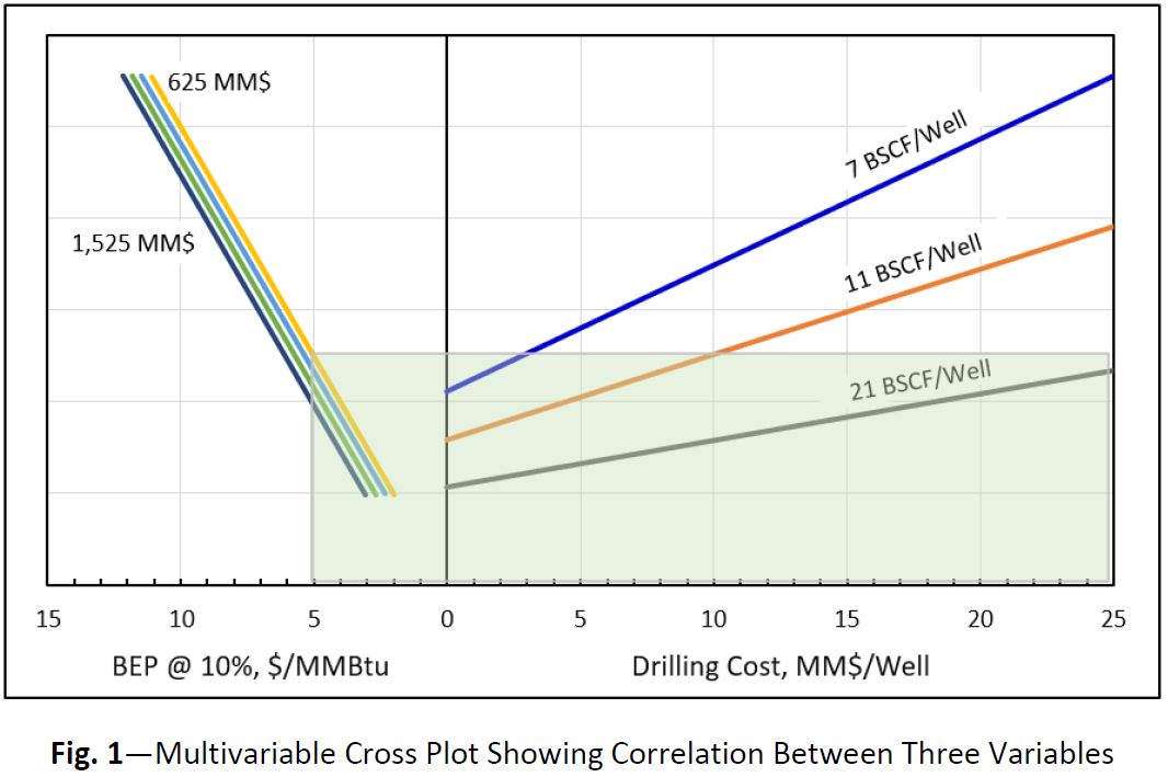
Fig. 1 instantly shows the feasible region of gas field development options. The figure shows that if the desired breakeven (BE) price of gas field development is $5/MMBtu and the CAPEX is $625 million then the field with 7 BSCF/well cannot be developed if the drilling cost is more than $3 million per well. Similarly, for the same BE price and facilities’ CAPEX the field with 11 BSCF/well potential cannot be developed if the drilling cost is more than $10 million per well. If the facilities’ CAPEX is increased to $1,525 million then then drilling cost cannot be more than $18 million per well even for a field with 21 BSCF/well potential.
Alternatively, the BE price can be determined for any drilling cost per well, reserves per well and facilities’ CAPEX. Fig. 2 shows that if the drilling cost per well is $15 million per well, field’s well potential is 11 BSCF/well and the facilities’ CAPEX is $1,525 million then the BE price of development will be $7.0/MMBtu.
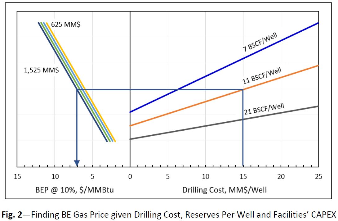
These types of plots are very handy in decision-making. Such plot can be used to give instant answers, even when in a meeting, without re-running the economics. The plots in Figures 1 and 2 show BE gas prices at a discount rate of 10%. The data in the second quadrant can be correlated with BE price at 10%, 12% and 15% discount rates in the third quadrant and so on. In the fourth quadrant, the before-tax and after-tax BE price may be shown.
Any other variables, beside the ones shown in Figure 1 & 2 can be correlated in similar way. The plots are not restricted to project economics, any problems where the outcome is affected by multiple variables can be plotted in the same way.
It is very simple to generate such plots. The following steps are followed to generate the multivariable cross plot.
- Step 1. Decide on the variables and the resulting profitability indicators (if the plot is intended to be used for field development economics) to be correlated.
- Step 2. Run sensitivities on the variables to be correlated. The sensitivities can be instantly generated using:
For the BE price calculation, the Data Table function of Excel and the following equation can be used (if before-tax economics are performed).
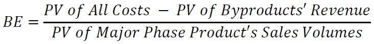
Major phase product will be sales gas in the gas field development and oil in the oil field development. The byproducts will be condensate, Ethane, Sulphur and NGLs as applicable. The BE price is also referred to as the Long-Range Marginal Cost (LRMC). Both the numerator and denominator have to be calculated at the same discount rate.
The above equation will not work for after-tax economics as the BE prices has to be calculated using the Excel’s Goal_Seek function. An Excel macro has to be built if BE price for after-tax economics has to be calculated.
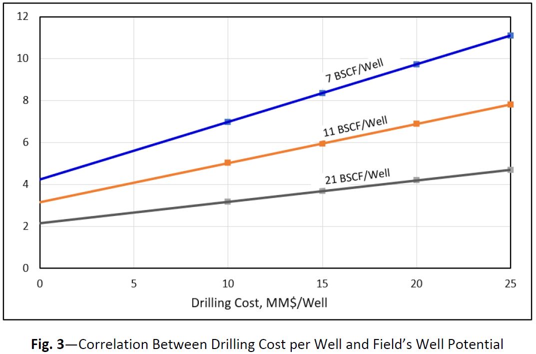
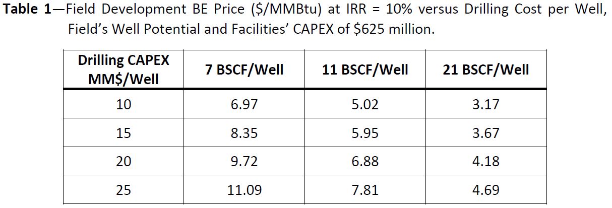
- Step 3. The BE prices at IRR = 10% are calculated at variable drilling costs per well and field’s well potential as shown in Table 1. This data is plotted as shown in the first quadrant of Fig. 3. These plots will normally plot as straight lines. Therefore, three to four points are enough to make sure they form a straight line. Trendline is fitted through each set of the data points so that the lines could be extended backward or forward (to cover a wider range) as desired.
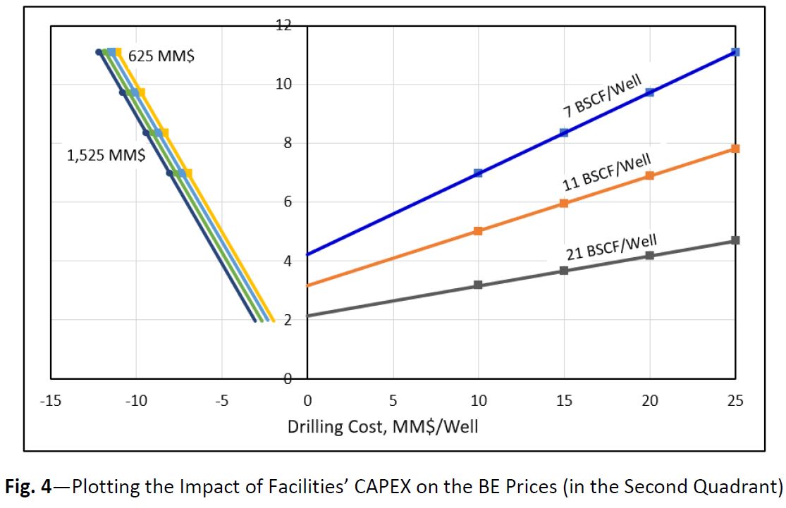
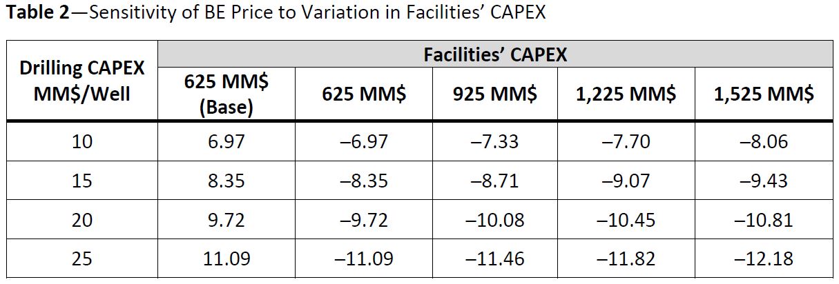
- Step 4. Generate the data to be plotted in the second quadrant of the graph. The BE price is now calculated for each drilling cost per well while changing the facilities’ CAPEX. The data in Table 1 is for the Base Facilities’ CAPEX of $625 million. Table 2 shows the BE price for CAPEX of $925, $1,225 and $1,525 million, respectively.
The BE price for the first quadrant is given on the Y-axis. The next set of BE prices will be plotted as negative BE prices on the X-axis (note that positive BE prices are calculated for this particular exercise but the sign is changed to negative for plotting). All these BE prices will be plotted against the existing BE prices on the Y-axis. The data of Table 2 is now added to the same graph as shown in Fig. 4.
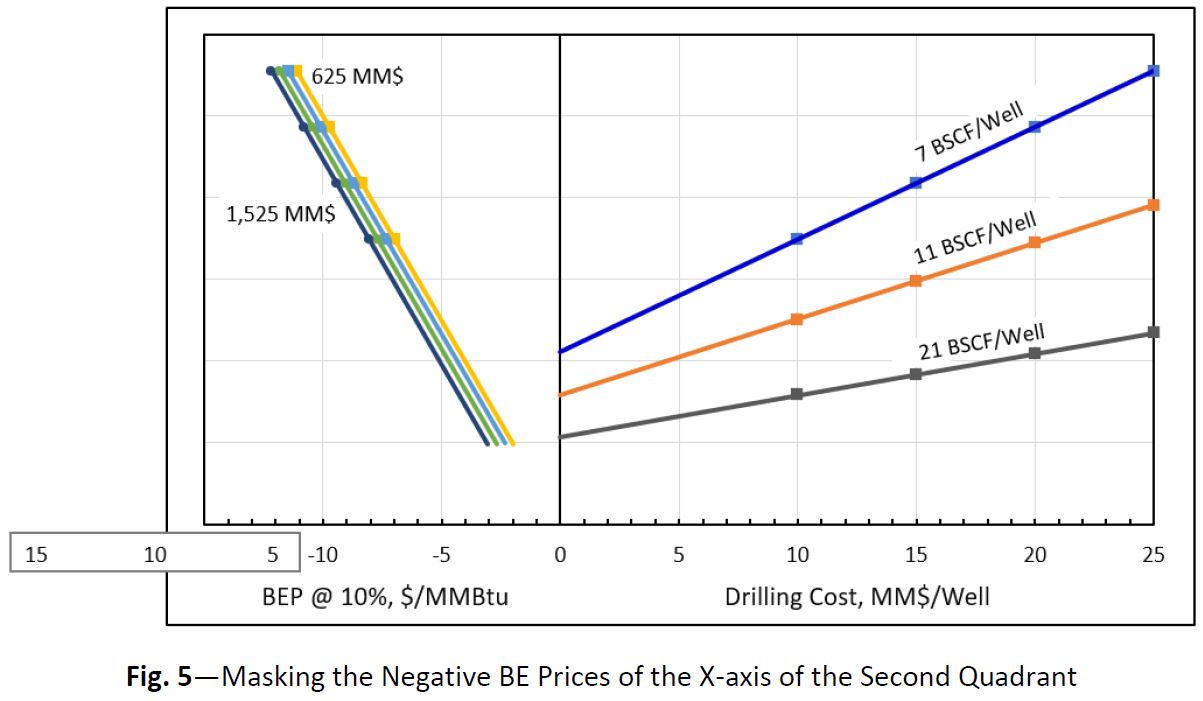
- Step 5. As negative BE prices are shown on the X-axis of the second quadrant, a small trick is required to change these to positive. Insert a shape (with white background fill and no line) and add positive axis labels to it as shown in Fig. 5. Drag the shape to the right so that all the negative BE pries are masked. Edit the X-axis title to add the BE price corresponding to the X-axis of the second quadrant.
- Step 6. The multivariable plot is now ready. The rest of the formatting can be done as desired. The final plot, after formatting, is as shown in Fig. 1. Randomly check the BE prices for various combinations from the plot with the BE prices calculated in the economics model to make sure the plot is giving correct answers.
References
- Mian, M. A., “Custom Graphs Help Analyze Oil, Gas Operations”, Oil & Gas Journal, October 20, 2003.
- Mian, M. A., Project Economics and Decision Analysis, Vol. 1 – Deterministic Models, PennWell Publishing Company, Tulsa, Oklahoma, USA, 2011.
A. Mian, registered professional engineer (PE) in the State of Colorado, is a principal consultant at O&G Knowledge Sharing Platform. Mian has 40 years of experience in reservoir engineering, project economics and strategic planning. He has a BS degree in mechanical engineering, an MS degree in petroleum engineering and an MS degree in mineral economics. Both the masters are from the Colorado School of Mines. Mian is the author of six books: Petroleum Engineering Handbook for the Practicing Engineers, Vol. 1 and 2, Project Economics and Decision Analysis, Vol. 1 and 2 and Tips & Tricks for Excel Based Financial Modeling, Vol. 1 and 2. The books on project economics and decision analysis are currently used as textbooks to teach project economics to graduate and undergraduate students in many universities worldwide. He has also published many technical papers and presented papers at SPE conferences. Mian has also delivered 5-day courses on reservoir engineering, project economics and decision analysis and advanced project economics and decision analysis in 25 countries.